[Originally published on June 9, 2014.]
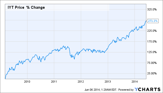
The transportation industry has benefited from a significant increase since its 2009 low, taking under consideration solely the iShares Dow Jones Transportation Average ETF (NYSEARCA:IYT). The fund has posted a cumulative surge in price of approximately 270% since its 2009 low of ~$40 per share. Intuitively, the question arises of whether the transportation fund's rally is soon to be over, or whether there exists any significant upside, which investors can ride to the top.
In order to answer this question, our investment thesis dissects IYT's price action into fundamental and technical components, which individually delve into potential price drivers and growth likelihood. Moreover, we calculate that the transportation ETF shows a potential upside between 10% and 25% from its June 2, 2014 closing price, with a weighted average price target of $170 per share for the end of 2014. Fundamentally, we believe that a continued slow pace in inflation (CPI), weakness in the trade-weighted value of the U.S. dollar, and a steady growth in real personal disposable income, will drive higher consumption in durable goods and a sharper increase in manufacturers' orders overall, in turn, causing a steady rise in the quantity of shipments (freight), while a more aggressive increase in freight price would offset rising fuel and labor costs. More specifically, we project revenue to grow at an average pace of 9% per year over the next five years, outpacing the growth of total costs, which we projected to be a little over 6% within the same time frame, thus giving way to a cumulative annual growth rate in earnings of approximately 20%. Our custom version of the abnormal earnings growth model implies a fair value (i.e. fair value for IYT Net Assets) of $1.343 Billion, or $182 per share, by the end of 2014. Using the same variables, but a different technique, we employ a direct time series regression, as a supplementary component of fundamental analysis (i.e. a secondary fundamental model), to derive expected annual return of 19% or a year-end price target of approximately $156 per share. From a technical perspective, price is currently in the higher-end of its oscillation cycle around a de-exponentialized 10-year trend line. History tells us that although at this point the security seems expensive, price lingers for a while around the higher-end of the oscillation channel before finally coming down. Hence, technical assessment implies a $160 per share price target by the end of 2014.
The Fundamental Approach
Quantity, Price, and Revenue
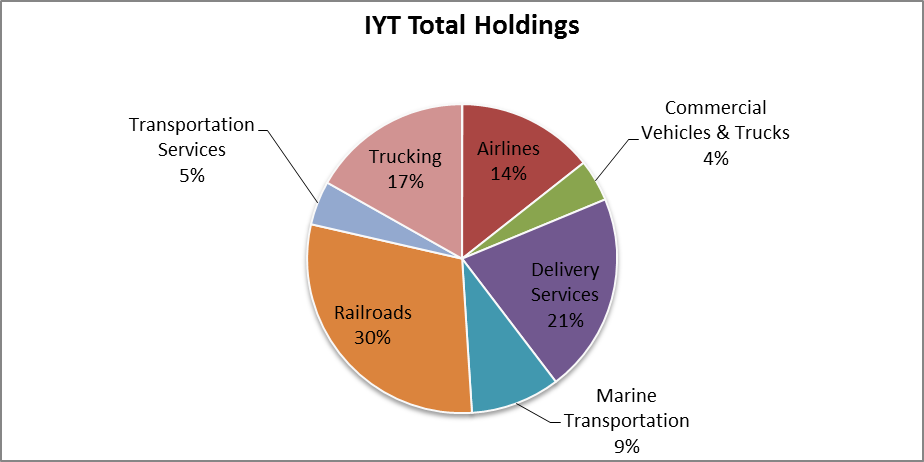
The transportation ETF's holdings suggest that IYT should more likely be named the "freight" ETF, as more than 86% of the fund's holdings are directly associated with the freight industry. Less than 14% of the entire portfolio is passenger-related, represented by the five airlines held by the ETF. Furthermore, it is important to consider airlines' cargo business component, as it is also embedded into the overall value of the ETF's airlines equity holdings, and contributes to the premise that IYT holdings represent, almost exclusively, the "freight" constituent of the transportation industry.
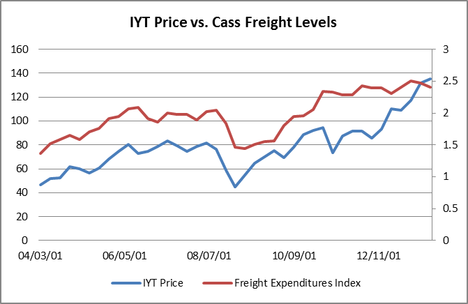
In that regard, we assume the growth of the industry would be highly correlated with, if not equivalent, to national freight and shipment indices measuring the quantity of shipments as well as total freight expenditures. More specifically, we single out the Cass Freight Indices as some of the most relevant freight industry progression indicators, measured against historical performance of the iShares Dow Jones Transportation Average ETF. When tested at lags 0 and 1, IYT's Year-over-Year price change has a 57% correlation and 73% correlation, respectively, with Cass Freight Expenditures Index Year-over-Year change. In other words, price leads freight expenditures by approximately 1 quarter, for two likely reasons: 1.) according to Cass Information Systems, "volumes represent the month in which transactions are processed by Cass, not necessarily the month when the corresponding shipments took place" and 2.) the market may show a certain ability to form somewhat accurate expectations of changes in freight levels. The evidently strong positive correlation between the ETF price performance and the change in Freight Expenditures, we attribute to the index's ability to track and represent the growth of the broad freight industry.
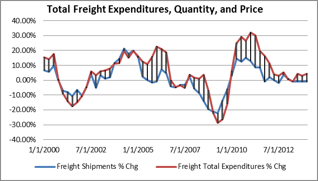
Along with the freight expenditures index, we also employ the Cass Freight Shipments Index as a representative of the quantity component behind the "Price x Quantity" function. In other words, the freight shipments index represents the quantity component of total revenue, while the price component is represented by backing out the change in quantity (freight shipments) from the change in total expenditures (freight expenditures). As exhibited in the graph below, the implied price change is represented by the shaded area between the two lines: Freight Shipments % Chg and Freight Total Expenditures % Chg.
Quantity growth of total shipments in the industry, represented by the change in levels of the Cass Freight Shipments Index, is driven by a series of macro variables such as inflation (measured by CPI),trade-weighted value of the U.S. dollar (measured by the FRB), real disposable income levels, Manufacturers' New Orders, price of freight (as derived by the methodology described in the previous paragraph), and cyclicality in the change of quantity. The method used for measuring variables' interdependence is a multivariate time series regression, specifically a Vector Autoregressive Model (quick overview here from Penn State), which expresses the interrelation of the described variables' rate of change through a system of equations estimating the respective dependent values as well as each variable's interrelation with each other variable.
In order to gauge predictive power of each variable, one of the pre-estimation tests/statistics we use is a bivariate correlogram to assist in identifying optimal lags/leads.
CPI's rate of change shows high negative correlation in subsequent lags, therefore suggesting that the quantity of shipments lags inflation and tends to begin deteriorating in periods following high inflation. Therefore, evidence suggests that as prices begin rising, the market can expect lower consumption of goods.
Inflation | |
Lag | Correlation |
0 | 0.2752 |
1 | 0.0224 |
2 | -0.2371 |
3 | -0.446 |
4 | -0.5397 |
5 | -0.5158 |
6 | -0.4297 |
7 | -0.3085 |
8 | -0.2378 |

The trade-weighted value of the dollar as calculated by the FRB, observes the major currencies involved in trade with the U.S. and indexes the U.S. dollar's value relative to those very currencies. We observe that the dollar value leads the quantity of shipments with a negative correlation implying that the quantity of shipments falls following a rise in the U.S. dollar value relative to the currencies of our major trade partners. Logic implies that as it become more expensive for foreigners to purchase U.S. goods, the quantity of goods purchased will fall, leading to a lower overall quantity of shipments.
Dollar Value | |
Lag | Correlation |
0 | -0.4761 |
1 | -0.4682 |
2 | -0.3801 |
3 | -0.2977 |
4 | -0.1794 |
5 | -0.0582 |
6 | 0.0307 |
7 | 0.0939 |
8 | 0.12 |

Real Disposable income exhibits the highest correlation in lags 0 and 1, which is positive, suggesting that an increase in real disposable income leads to an increase in quantity of shipments in current quarters. Logic gives way to the explanation that as income rises, so does consumption, which then spills over to an increase in freight and shipment.
Disposable Income | |
Lag | Correlation |
0 | 0.3898 |
1 | 0.3285 |
2 | 0.0916 |
3 | -0.0952 |
4 | -0.1957 |
5 | -0.2853 |
6 | -0.2525 |
7 | -0.2481 |
8 | -0.205 |

Implied price of freight exhibits the strongest correlation with freight quantity at lags 3 and 4, which is negative, and somewhat supports popular theory that as price rises, quantity falls, and vice versa. However, the high number of lags here suggests more of a cyclical pattern, rather than end-user response to price. In other words, once price change has substantially accelerated, it most likely signals "overheating" in freight and consumption, leading us to expect a downturn in quantity as a future response. In other words, the price cycle holds some information regarding the quantity cycle. The more interesting relationship is how quantity leads price, which will be covered further into the report.
Price of Freight | |
Lag | Correlation |
0 | 0.2021 |
1 | 0.0869 |
2 | -0.0917 |
3 | -0.2292 |
4 | -0.2185 |
5 | -0.1925 |
6 | -0.1015 |
7 | -0.0467 |
8 | -0.0705 |

Manufacturers' new orders exhibits the strongest correlation with freight quantity at lags 2 and 3. The correlations are positive, indicating that manufacturers' new orders lead the quantity of shipments. This works in two ways: 1.) as manufacturers submit orders, shipping lags as delivery takes some time depending on the supply chain complexity and efficiency and 2.) manufacturers signal an increase in demand for consumption of tangible goods, thus implying a rise in deliveries and shipments in subsequent quarters.
Manufacturers' new Orders | |
Lag | Correlation |
0 | 0.0789 |
1 | 0.3876 |
2 | 0.5602 |
3 | 0.5132 |
4 | 0.4471 |
5 | 0.2895 |
6 | 0.1509 |
7 | 0.1063 |
8 | 0.0638 |

Without getting into the technical details of post-estimation tests and test statistics, we display the back-tested results (i.e. the values predicted by the model versus the actual historical values). The sample size displayed, for the purpose of visual ease, includes 56 observations, as the time series are set in quarterly intervals.
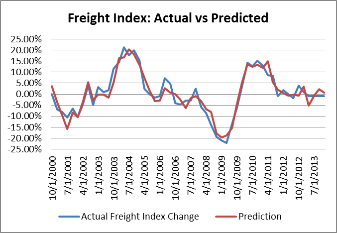
Based on the progression of the variables simulated by the system of estimated equations, we estimate the impact of each variable on the change of quantity of shipments. The chart showing each factor's contribution portrays the impact somewhat simplistically, as variables' evolution through time does not only impact quantity, but rather it impacts every other variable, which in turn, additionally spills over to affect the change in quantity of shipments. For example, while a rise in disposable income causes a rise in quantity of shipments, it also causes a rise in inflation, which in turn, affects quantity negatively, possibly even offsetting the positive direct effect that a rising in disposable income has on freight quantity.
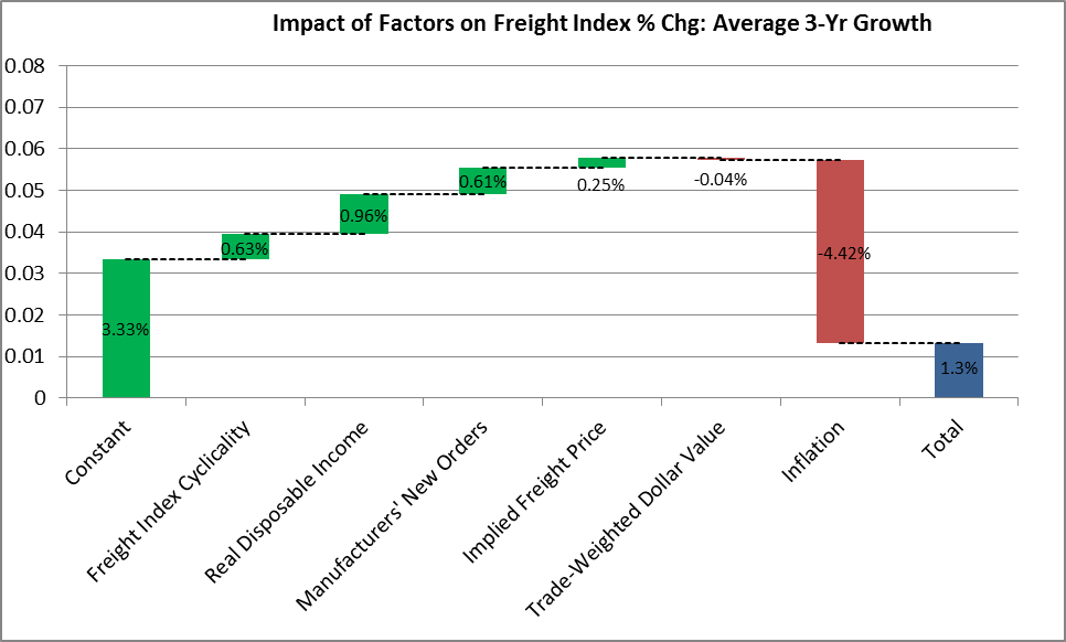
We see a steady rise in disposable income, manufacturers' new orders, and the index's cyclical tendencies to be the main tailwinds pushing freight quantity upward, while we expect a steady rising inflation (average of 2.2% year-over-year over the next 3 years) to drag down the quantity of shipments to an average annual growth rate of 1.3% over the next three years. This projected growth is a little higher than the 16-year average Year-over-Year growth in the freight index of 0.8%.
Date | Freight Index |
4/1/2014 | 3.99% |
7/1/2014 | -1.51% |
10/1/2014 | 0.89% |
1/1/2015 | 0.72% |
4/1/2015 | -0.14% |
7/1/2015 | 1.30% |
10/1/2015 | 0.58% |
1/1/2016 | 0.70% |
4/1/2016 | 1.59% |
7/1/2016 | 1.88% |
10/1/2016 | 2.70% |

Price growth in the freight industry, as mentioned earlier, is derived from quantity of freight shipments and total freight expenditures solving for dP=dR/dQ, where P represents the implied price, Rrepresents total freight expenditures, and Q represents the quantity of freight shipments. When analyzing implied price, it is important to keep in mind that via the derivation method, freight price changes account for the change in total ton-miles in the industry. Furthermore, like quantity, price is part of the system of equations and is affected by the endogenous variables within the system as well as exogenous inputs, described in the quantity section. However, as expected, price responds somewhat differently to the same system of variables than quantity.
Inflation is both coincident and leads freight price by one quarter as the strongest correlation is exhibited at lags 0 and 1. The positive correlation implies that as general price increase occurs in the economy, the freight industry follows the trend of rising pricing. In other words, as consumption begins overheating, causing consumer prices to rise, the price of shipping soon follows.
Inflation | |
Lag | Correlation |
0 | 0.509 |
1 | 0.5147 |
2 | 0.292 |
3 | -0.0196 |
4 | -0.3135 |
5 | -0.4558 |
6 | -0.4493 |
7 | -0.3635 |
8 | -0.1943 |

The change in the U.S. dollar value's strongest correlation with the change in the freight price occurs in lags 1-3. In other words, changes in the value of the dollar lead the change in freight rates with a negative relationship. In a hypothetical scenario where the dollar increases in value relative to the currencies of the United States' major trade partners, this will lead to a decline in foreign purchases of U.S. goods, a decline in exports, and, consequently, a decline in shipping quantity as well as a decline in shipping price.
Dollar Value | |
Lag | Correlation |
0 | -0.0998 |
1 | -0.3614 |
2 | -0.4634 |
3 | -0.3515 |
4 | -0.1681 |
5 | -0.0077 |
6 | 0.075 |
7 | 0.0635 |
8 | -0.0044 |

The relationship between disposable income and freight rates is a quite interesting one, as we observe that disposable income has a negative leading relationship with price. Hence, if disposable income increases, one can expect prices to fall in subsequent quarters. However, looking at the relationship between quantity and disposable income, we observe that freight quantity increases as disposable income rises. Hence, the number of possible logical explanations that support this empirical relationship is limited to a supply-side assumption. In other words, we attribute this negative relationship between a disposable income and freight price to supply-side "price pressures," or companies within the sector cutting prices (under-bidding) in an attempt to capture market share. Here is how we see the chronology/cycle developing: as disposable income rises, at moderate prices, it causes a rise in quantity of freight on the demand side, therefore beginning to subsequently push prices higher; after quantity has been rising (and subsequently prices) the freight industry enters a later stage of the cycle where quantity demanded is not accelerating at the same rate, thus forcing competition within the industry to fight for market share by slashing prices and trying to out-bid the competition, in turn keeping a floor under quantity growth via the price mechanism. This would be a text-book development of a self-correcting market/industry where the forces of competition drive development (as the founders of capitalism would remark). The competition most likely occurs in the trucking sub-industry, among other sub-industries, as it is one of the most competition-susceptible sub-industries in the freight industry.
Disposable Income | |
Lag | Correlation |
0 | 0.1663 |
1 | -0.0041 |
2 | -0.0934 |
3 | -0.2771 |
4 | -0.3434 |
5 | -0.2891 |
6 | -0.2528 |
7 | -0.1116 |
8 | -0.0579 |

Freight quantity, is an evident and a stronger leader of freight price than price is of quantity. Quantity leads price by 1-3 quarters with a strong positive correlation, implying that increases in quantity cause an increase in freight rates as well. The opposite would also be true, as quantity declines, freight companies will have threshold where they will not trade price for a marginal increase in freight tonnage or units with the purpose of optimizing revenue amount. However, in very slow or recessionary periods, a price decrease would follow a decrease in freight quantity, as firms would attempt to maintain an adequate return on assets.
Freight Index | |
Lag | Correlation |
0 | 0.2021 |
1 | 0.3675 |
2 | 0.3865 |
3 | 0.3685 |
4 | 0.3302 |
5 | 0.1749 |
6 | 0.1013 |
7 | -0.0024 |
8 | -0.0705 |

Similar to our approach in measuring/forecasting quantity, we offer visual results that allow for gauging the proximity of our VAR model predictions to the actual change in freight rates.
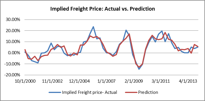
In assessing the drivers' impact on three-year average year-over-year change in freight price, as illustrated in the waterfall chart below, we see the only negative contributor being changes in real disposable income, as the freight industry will be entering into a new phase of the cycle, thus beginning to show limited effects of competitive pricing. One indirect relationship that is not illustrated by the chart below, however, is real disposable incomes' tendency to lead inflation. In other words, steady increasing disposable income leads a steady increase in inflation, thus causing an overall increase in prices for goods as well as shipping prices.

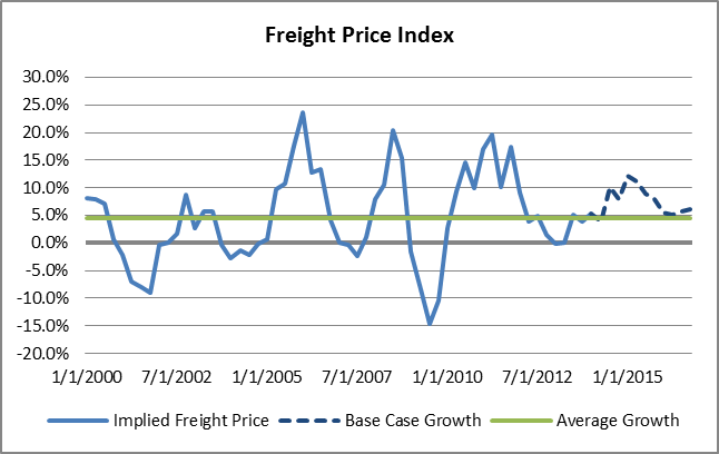
According to our study, the only headwinds to freight rate/price increases are attributable to real disposable income as it predicts some price pressures from competition. However, price cyclicality, steady inflation, and a rise in manufacturers' orders along with freight quantity, amount to an average year-over-year change in implied freight price of 7.6% for the next three years. This is approximately 3% higher than the 16-year average YoY change in freight price/rates of 4.6%.
Date | Price Growth |
4/1/2014 | 3.81% |
7/1/2014 | 10.06% |
10/1/2014 | 7.98% |
1/1/2015 | 12.17% |
4/1/2015 | 11.21% |
7/1/2015 | 8.89% |
10/1/2015 | 7.85% |
1/1/2016 | 5.44% |
4/1/2016 | 5.09% |
7/1/2016 | 5.68% |
10/1/2016 | 6.13% |
Revenue in the freight industry, of course, is a function of quantity and price, and in turn, it is equivalent to the growth of total freight expenditures in our view. We expect that average YoY growth in revenue over the next 3 years will be around 8.8%, which is right in line with the average industry revenue growth in the last 4 years. It is important to note, that when mentioning "industry", we mean the sum of the revenue of all of IYT's holdings.
Quarterly Revenue | |||
Date | Quantity Growth | Price Growth | Revenue Growth |
4/1/2014 | 3.99% | 3.81% | 7.96% |
7/1/2014 | -1.51% | 10.06% | 8.40% |
10/1/2014 | 0.89% | 7.98% | 8.94% |
1/1/2015 | 0.72% | 12.17% | 12.98% |
4/1/2015 | -0.14% | 11.21% | 11.05% |
7/1/2015 | 1.30% | 8.89% | 10.30% |
10/1/2015 | 0.58% | 7.85% | 8.47% |
1/1/2016 | 0.70% | 5.44% | 6.18% |
4/1/2016 | 1.59% | 5.09% | 6.77% |
7/1/2016 | 1.88% | 5.68% | 7.66% |
10/1/2016 | 2.70% | 6.13% | 8.99% |
Annual Revenue | |||
Date | Quantity Growth | Price Growth | Revenue Growth |
10/1/2014E | 0.89% | 7.98% | 8.94% |
10/1/2015E | 0.58% | 7.85% | 8.47% |
10/1/2016E | 2.70% | 6.13% | 8.99% |
Costs: Cost of Revenue and Other Operating Costs
Our costs analysis begins with research from the "Freight Rate Index" where costs of freight are broken down into individual components contributing to costs per mile. Monthly editions are released tracking the absolute value of freight costs/rates as well as cost components' percentage of the total. The index applies to "freight transport by land" and in terms of freight tonnage, assumes a full-loaded 48 foot trailer with a standard long-haul semi-tractor unit, all applicable to the trucking industry.


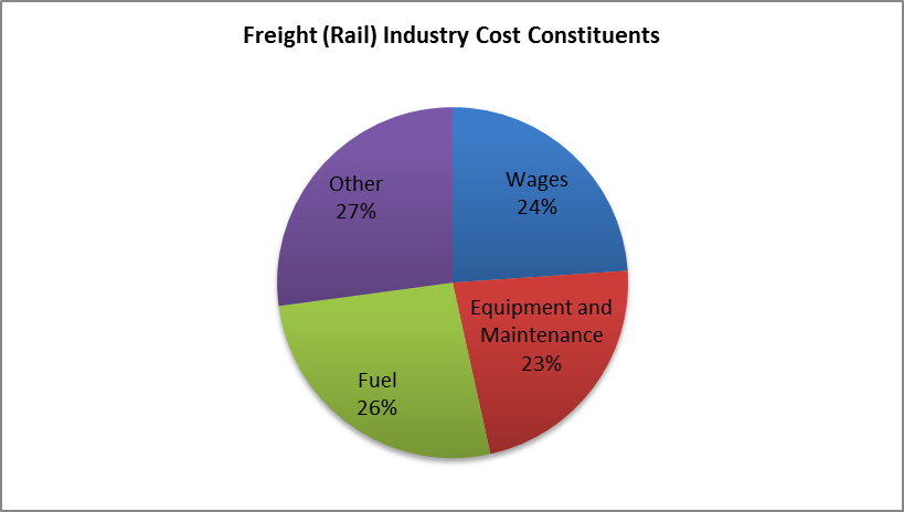
We also gather data from the Surface Transportation Board in order to examine the cost components of the railroad industry, which represents approximately 30% of the iShares Dow Jones Transportation Average ETF holdings. We average the four-year aggregated operating expense components as a percentage of total operating expenses of seven railroad companies, and categorize them by type.
We apply the same methodology to the delivery sub-industry which includes FedEx, UPS, and Expeditors International. In order to derive costs by component, we review the annual financial reports and compile reported costs by category.
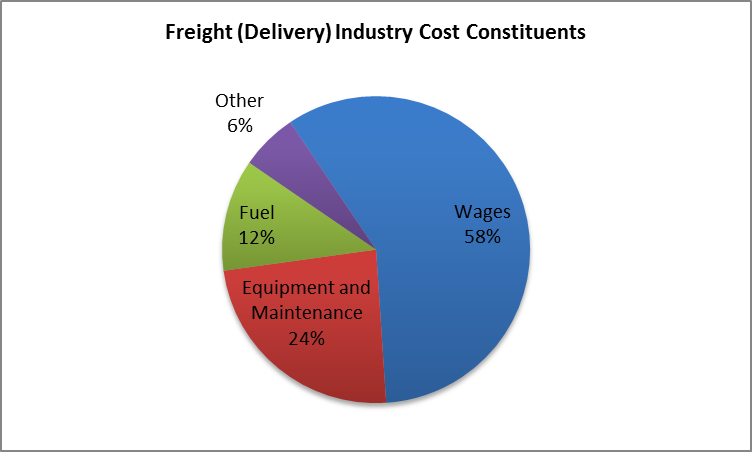
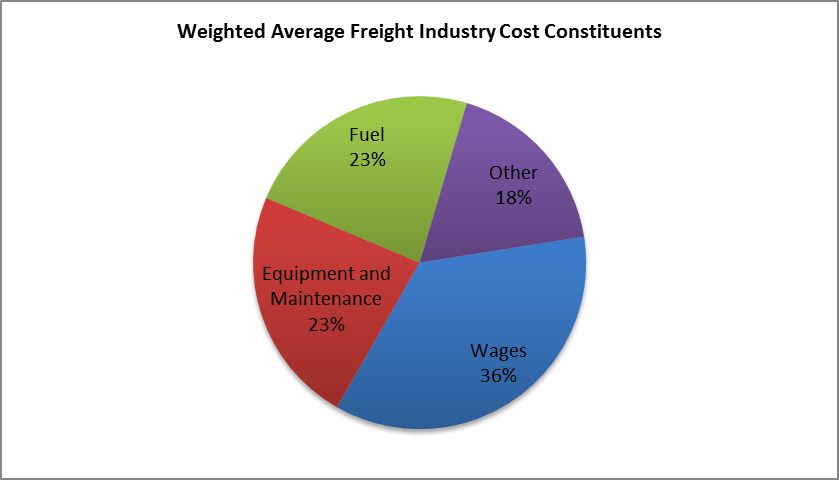
The three sub industries represent more than 2/3 of the entire ETF holding, with a mild variation in the percentage-of-the-total cost component allocation. We aggregate the cost component allocations via a weighted average, using the portion of shares held by the ETF adjusted by the portion of the industry that each company represents.
Fuel costs are represented by the BLS' "Fuels & Related Products" PPI Index, which we adjust to exclude coal products, industrial electric power, and home heating oils and distillates. Furthermore, we use an adjustment factor relative to implied freight price in order to account for ton-miles, or in certain cases, for Forty-Foot Equivalents.
Date | Producer Price Index: Fuels & Related Products |
4/1/2014 | 8.18% |
7/1/2014 | 11.49% |
10/1/2014 | 14.56% |
1/1/2015 | 15.59% |
4/1/2015 | 14.02% |
7/1/2015 | 11.51% |
10/1/2015 | 8.39% |
1/1/2016 | 6.23% |
4/1/2016 | 5.78% |
7/1/2016 | 6.47% |
10/1/2016 | 7.31% |

Equipment and Maintenance cost growth is derived from the "Manufacturers' Shipments for Durable Goods Industries: Transportation Equipment." The interesting relationship between transportation equipment shipments and freight companies is that, essentially, logic indicates that freight companies ship equipment to themselves, therefore the industry as a whole should not be affected by shipping costs for new equipment, but rather the manufacturers' price.
Another fact is the interdependency between freight quantity and transportation equipment shipments: as freight quantity increases, the need for transportation equipment and capital expenditures increase, and at the same time, when new transportation equipment is purchased, freight quantity also rises, as that new equipment needs to be shipped. Thus, we link equipment and maintenance to our system of equations described earlier.
.
Date | Manufacturers' Shipments for Durable Goods Industries: Transportation Equipment |
4/1/2014 | 2.19% |
7/1/2014 | 1.84% |
10/1/2014 | 3.08% |
1/1/2015 | 4.31% |
4/1/2015 | 4.95% |
7/1/2015 | 4.78% |
10/1/2015 | 3.92% |
1/1/2016 | 3.14% |
4/1/2016 | 2.84% |
7/1/2016 | 3.09% |
10/1/2016 | 3.51% |
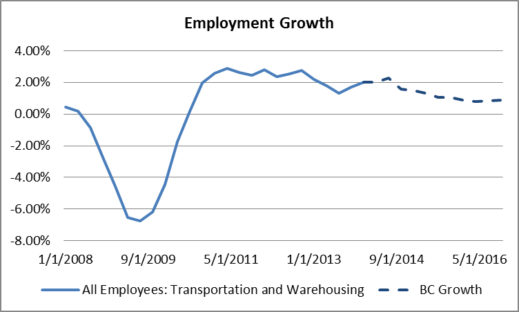
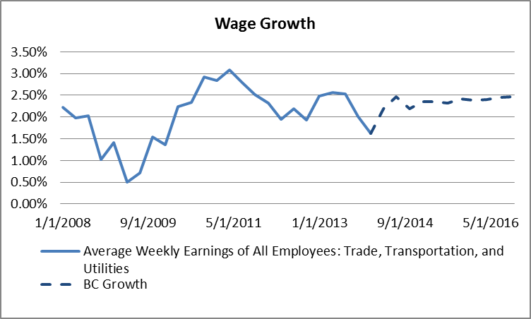
Wages are estimated as a function of the quantity of employees and the average wage paid. We find that the change in quantity of employees in the transportation industry, is heavily related to the change in quantity of freight and the change in average wages. Hence, along with transportation equipment, we link wages to the system of equations which drives the progression of each variable through time. Based on quantity and wage progression we assume that quantity of employees in the industry will increase marginally, surpassed by the growth in wages. Rising wages, and shortage of drivers, has been the trend for more than 3 years in the trucking industry, as we expect that this sub-industry will be the main driver of labor quantity-wage trade-off.
Date | All Employees: Transportation and Warehousing | Average Weekly Earnings of Employees |
4/1/2014 | 2.00% | 2.19% |
7/1/2014 | 2.26% | 2.46% |
10/1/2014 | 1.56% | 2.19% |
1/1/2015 | 1.50% | 2.35% |
4/1/2015 | 1.32% | 2.35% |
7/1/2015 | 1.06% | 2.33% |
10/1/2015 | 1.05% | 2.42% |
1/1/2016 | 0.90% | 2.39% |
4/1/2016 | 0.80% | 2.40% |
7/1/2016 | 0.84% | 2.46% |
10/1/2016 | 0.86% | 2.47% |
Date | All Employees: Transportation and Warehousing | Producer Price Index: Fuels & Related Products | Manufacturers' Shipments for Durable Goods Industries: Transportation Equipment | Average Weekly Earnings of Employees |
10/1/2014E | 1.56% | 14.56% | 3.08% | 2.19% |
10/1/2015E | 1.05% | 8.39% | 3.92% | 2.42% |
10/1/2016E | 0.86% | 7.31% | 3.51% | 2.47% |
Where applicable, we adjust the change in costs by the change in quantity in order to arrive at total spend per input. The total expenditures are organized into a matrix, displaying year-over-year growth, as the growth rates are in turn mapped and applied to the freight industry's aggregate financials. After 2016, we assume a constant growth in both, costs and revenue, equivalent to the growth estimated in 2016.
Costs in % | ||||||
2014 | 2015 | 2016 | 2017 | 2018 | 2019 | |
Total Costs | 7.3% | 5.7% | 6.2% | 6.3% | 6.4% | 6.5% |
Cost of Revenue | 8.0% | 5.8% | 6.2% | 6.3% | 6.4% | 6.6% |
Fuel | 15.6% | 9.0% | 10.2% | 10.2% | 10.2% | 10.2% |
Labor | 3.8% | 3.5% | 3.4% | 3.4% | 3.4% | 3.4% |
Equipment | 3.1% | 3.9% | 3.5% | 3.5% | 3.5% | 3.5% |
Operating Costs | 5.1% | 5.1% | 6.1% | 6.1% | 6.1% | 6.1% |
Depreciation | 6.5% | 6.5% | 6.5% | 6.5% | 6.5% | 6.5% |
SG&A | 3.1% | 3.0% | 5.2% | 5.2% | 5.2% | 5.2% |
Other | 6.9% | 6.9% | 6.9% | 6.9% | 6.9% | 6.9% |
Revenue | 8.9% | 8.5% | 9.0% | 9.0% | 9.0% | 9.0% |
Income Statement and Valuation
The fundamental approach we take to valuing the fund's portfolio is a blend of methods including a custom variation of the AEG Model and, to a lesser extent, a sum-of-the-parts method. In other words, we compile and aggregate the financial performance (income statements) of all of the ETF portfolio's holdings assuming that it represents the entire industry, and to it we apply the growth rates calculated, which are represented in the table above. The finer print of the methodology lies within the aggregation methods of the industry's income statement. In order to aggregate the industry's financials, we add the income statement line items of all holdings, weighted by the amount of shares held by IYT as a percentage of each respective company's total shares outstanding. This method allows us to treat the industry as a single firm, which is exposed to the business environment of all of its components, in essence being comparable to a parent company with multiple subsidiaries in a single industry. To reinforce this assumption, we sum the market cap of each of IYT's holdings weighted by the amount of shares held by IYT as a percentage of each respective company's total outstanding shares. The result is almost equivalent to IYT's net asset value, within 1% variability.
The first table (below) shows the plain sum of all of IYT's holdings' income statement line items, without any adjustments or weightings applied, for the past four years.
Total Industry Income (in millions $) | 2013 | 2012 | 2011 | 2010 |
Revenue | $295,852.51 | $285,255.35 | $273,235.81 | $231,755.20 |
Other Revenue, Total | $0.00 | $0.00 | $0.00 | $0.00 |
Total Revenue | $295,852.51 | $285,255.35 | $273,235.81 | $231,755.20 |
Cost of Revenue, Total | $198,520.14 | $199,628.64 | $179,211.70 | $146,687.48 |
Gross Profit | $97,332.36 | $85,626.72 | $94,024.13 | $85,067.70 |
Selling/General/Admin. Expenses, Total | $26,796.92 | $25,860.07 | $32,143.96 | $29,720.98 |
Research & Development | $0.00 | $0.00 | $0.00 | $0.00 |
Depreciation/Amortization | $14,032.61 | $13,256.89 | $12,497.91 | $11,626.96 |
Interest Expense(Income) - Net Operating | $0.00 | $0.00 | $0.00 | $0.00 |
Unusual Expense (Income) | $1,789.86 | $2,201.18 | $1,185.69 | $1,643.57 |
Other Operating Expenses, Total | $19,896.41 | $18,882.87 | $18,495.09 | $16,316.03 |
Total Operating Expense | $259,357.01 | $258,398.15 | $242,141.74 | $205,995.00 |
Operating Income | $34,958.57 | $25,393.90 | $29,710.06 | $25,760.16 |
Interest Income(Expense), Net Non-Operating | $0.00 | $0.00 | $0.00 | $0.00 |
Gain (Loss) on Sale of Assets | $314.77 | $197.61 | $203.68 | $135.83 |
Other, Net | $77.66 | $226.49 | -$74.76 | $60.86 |
Income Before Tax | $31,135.35 | $21,741.92 | $24,920.59 | $21,088.12 |
Income After Tax | $28,952.36 | $13,975.86 | $16,608.30 | $13,509.80 |
Minority Interest | -$6.63 | -$4.89 | -$4.63 | -$0.03 |
Equity In Affiliates | $75.80 | $19.60 | $32.40 | $28.50 |
Net Income Before Extra. Items | $29,021.54 | $13,990.57 | $16,636.08 | $13,538.27 |
Accounting Change | $0.00 | $0.00 | $0.00 | $0.00 |
Discontinued Operations | $0.00 | -$6.10 | -$11.60 | $0.00 |
Extraordinary Item | $0.00 | $0.00 | $0.00 | $0.00 |
Net Income | $29,053.22 | $13,996.76 | $16,624.36 | $13,531.83 |
Preferred Dividends | $0.00 | $0.00 | $0.00 | $0.00 |
Income Available to Common Excl. Extra Items | $29,011.34 | $13,974.08 | $16,606.51 | $13,515.38 |
Income Available to Common Incl. Extra Items | $29,043.03 | $13,986.37 | $16,606.39 | $13,508.94 |
Basic Weighted Average Shares | $0.00 | $0.00 | $0.00 | $0.00 |
Basic EPS Excluding Extraordinary Items | $0.00 | $0.00 | $0.00 | $0.00 |
Basic EPS Including Extraordinary Items | $0.00 | $0.00 | $0.00 | $0.00 |
Dilution Adjustment | $37.70 | $14.00 | $47.31 | $43.00 |
Diluted Weighted Average Shares | 6,298.56 | 6,342.98 | 6,527.62 | 6,481.20 |
Diluted EPS Excluding Extraordinary Items | $76.49 | $53.37 | $51.84 | $39.32 |
Diluted EPS Including Extraordinary Items | $0.00 | $0.00 | $0.00 | $0.00 |
Total Dividends | $5,877.75 | $5,674.35 | $4,611.96 | $4,056.53 |
Growth Rates | 2013 | 2012 | 2011 |
Revenue | 4% | 4% | 18% |
Other Revenue, Total | |||
Total Revenue | 4% | 4% | 18% |
Cost of Revenue, Total | -1% | 11% | 22% |
Gross Profit | 14% | -9% | 11% |
Selling/General/Admin. Expenses, Total | 4% | -20% | 8% |
Research & Development | |||
Depreciation/Amortization | 6% | 6% | 7% |
Interest Expense(Income) - Net Operating | |||
Unusual Expense (Income) | -19% | 86% | -28% |
Other Operating Expenses, Total | 5% | 2% | 13% |
Total Operating Expense | 0% | 7% | 18% |
Operating Income | 38% | -15% | 15% |
Interest Income(Expense), Net Non-Operating | |||
Gain (Loss) on Sale of Assets | 59% | -3% | 50% |
Other, Net | -66% | -403% | -223% |
Income Before Tax | 43% | -13% | 18% |
Income After Tax | 107% | -16% | 23% |
Minority Interest | 36% | 6% | 15333% |
Equity In Affiliates | 287% | -40% | 14% |
Net Income Before Extra. Items | 107% | -16% | 23% |
Accounting Change | |||
Discontinued Operations | -100% | -47% | |
Extraordinary Item | |||
Net Income | 108% | -16% | 23% |
Preferred Dividends | |||
Income Available to Common Excl. Extra Items | 108% | -16% | 23% |
Income Available to Common Incl. Extra Items | 108% | -16% | 23% |
Basic Weighted Average Shares | |||
Basic EPS Excluding Extraordinary Items | |||
Basic EPS Including Extraordinary Items | |||
Dilution Adjustment | 169% | -70% | 10% |
Diluted Weighted Average Shares | -1% | -3% | 1% |
Diluted EPS Excluding Extraordinary Items | 43% | 3% | 32% |
Diluted EPS Including Extraordinary Items | |||
Total Dividends | 4% | 23% | 14% |
Stepping aside from the unadjusted sum of total IYT holdings' income statement line items, we move into the sum of the holdings' financials weighted by percentage of shares from the respective company's total outstanding shares held by the ETF portfolio. As mentioned above, this method allows us to treat the ETF as a parent holding company with a particular allocation/stake in individual "subsidiaries", all of which are in a single industry, and also gives us the ability to derive fair value using the performance of earnings and dividends.
Total ETF Income (in millions $) | 2010 | 2011 | 2012 | 2013 |
Revenue | $554.72 | $672.73 | $709.99 | $737.82 |
Other Revenue, Total | $0.00 | $0.00 | $0.00 | $0.00 |
Total Revenue | $554.72 | $672.73 | $709.99 | $737.82 |
Cost of Revenue, Total | $362.82 | $456.53 | $494.23 | $501.81 |
Gross Profit | $191.90 | $216.20 | $215.76 | $236.01 |
Selling/General/Admin. Expenses, Total | $77.39 | $84.30 | $80.65 | $83.39 |
Research & Development | $0.00 | $0.00 | $0.00 | $0.00 |
Depreciation/Amortization | $25.29 | $27.39 | $29.18 | $31.36 |
Interest Expense(Income) - Net Operating | $0.00 | $0.00 | $0.00 | $0.00 |
Unusual Expense (Income) | $2.60 | $2.09 | $3.39 | $3.58 |
Other Operating Expenses, Total | $34.98 | $38.94 | $39.80 | $42.56 |
Total Operating Expense | $503.08 | $609.25 | $647.24 | $662.70 |
Operating Income | $51.64 | $63.47 | $62.75 | $75.12 |
Interest Income(Expense), Net Non-Operating | $0.00 | $0.00 | $0.00 | $0.00 |
Gain (Loss) on Sale of Assets | $0.93 | $1.61 | $1.98 | $2.28 |
Other, Net | $0.15 | -$0.12 | $0.22 | -$0.03 |
Income Before Tax | $52.72 | $64.97 | $64.96 | $77.38 |
Income After Tax | $34.27 | $42.23 | $42.22 | $50.30 |
Minority Interest | $0.00 | -$0.04 | -$0.05 | -$0.05 |
Equity In Affiliates | $0.39 | $0.44 | $0.27 | $1.04 |
Net Income Before Extra. Items | $34.66 | $42.64 | $42.44 | $51.28 |
Accounting Change | $0.00 | $0.00 | $0.00 | $0.00 |
Discontinued Operations | $0.00 | -$0.18 | -$0.10 | $0.00 |
Extraordinary Item | $0.00 | $0.00 | $0.00 | $0.00 |
Net Income | $34.66 | $42.45 | $42.35 | $51.28 |
Preferred Dividends | $0.00 | $0.00 | $0.00 | $0.00 |
Income Available to Common Excl. Extra Items | $34.66 | $42.45 | $42.35 | $51.28 |
Income Available to Common Incl. Extra Items | $34.60 | $42.46 | $42.48 | $51.77 |
Basic Weighted Average Shares | $0.00 | $0.00 | $0.00 | $0.00 |
Basic EPS Excluding Extraordinary Items | $0.00 | $0.00 | $0.00 | $0.00 |
Basic EPS Including Extraordinary Items | $0.00 | $0.00 | $0.00 | $0.00 |
Dilution Adjustment | $0.14 | $0.11 | $0.04 | $0.08 |
Diluted Weighted Average Shares | 13.50 | 13.64 | 13.38 | 13.34 |
Diluted EPS Excluding Extraordinary Items | $39.32 | $51.84 | $53.37 | $76.49 |
Diluted EPS Including Extraordinary Items | $0.00 | $0.00 | $0.00 | $0.00 |
Total Dividends | $5.87 | $8.07 | $11.37 | $8.61 |
Growth Rates | 2011 | 2012 | 2013 | |
Revenue | 21% | 6% | 4% | |
Other Revenue, Total | ||||
Total Revenue | 21% | 6% | 4% | |
Cost of Revenue, Total | 26% | 8% | 2% | |
Gross Profit | 13% | 0% | 9% | |
Selling/General/Admin. Expenses, Total | 9% | -4% | 3% | |
Research & Development | ||||
Depreciation/Amortization | 8% | 7% | 7% | |
Interest Expense(Income) - Net Operating | ||||
Unusual Expense (Income) | -20% | 62% | 6% | |
Other Operating Expenses, Total | 11% | 2% | 7% | |
Total Operating Expense | 21% | 6% | 2% | |
Operating Income | 23% | -1% | 20% | |
Interest Income(Expense), Net Non-Operating | ||||
Gain (Loss) on Sale of Assets | 73% | 23% | 15% | |
Other, Net | -179% | -291% | -112% | |
Income Before Tax | 23% | 0% | 19% | |
Income After Tax | 23% | 0% | 19% | |
Minority Interest | -2398% | 20% | 13% | |
Equity In Affiliates | 14% | -40% | 287% | |
Net Income Before Extra. Items | 23% | 0% | 21% | |
Accounting Change | ||||
Discontinued Operations | -47% | -100% | ||
Extraordinary Item | ||||
Net Income | 22% | 0% | 21% | |
Total Dividends | 37% | 41% | -24% | |
Payout Ratio | 17% | 19% | 27% | 17% |
To the aggregated pro-forma statement, we apply the estimated growth rates in costs and revenue, in order to forecast earnings and dividends over a five-year horizon.
Total ETF Income (in millions $) | 2014E | 2015E | 2016E | 2017E | 2018E | 2019E |
Revenue | $803.82 | $871.92 | $950.33 | $1,035.78 | $1,128.92 | $1,230.43 |
Other Revenue, Total | ||||||
Total Revenue | $803.82 | $871.92 | $950.33 | $1,035.78 | $1,128.92 | $1,230.43 |
Cost of Revenue, Total | $542.08 | $573.66 | $609.43 | $648.07 | $689.84 | $735.05 |
Gross Profit | $261.73 | $298.26 | $340.90 | $387.71 | $439.08 | $495.38 |
Selling/General/Admin. Expenses, Total | $85.97 | $88.56 | $93.19 | $98.07 | $103.20 | $108.61 |
Research & Development | ||||||
Depreciation/Amortization | $33.39 | $35.55 | $37.85 | $40.30 | $42.91 | $45.68 |
Interest Expense(Income) - Net Operating | ||||||
Unusual Expense (Income) | ||||||
Other Operating Expenses, Total | $45.52 | $48.67 | $52.05 | $55.66 | $59.53 | $63.66 |
Total Operating Expense | $706.96 | $746.44 | $792.52 | $842.10 | $895.48 | $953.00 |
Operating Income | $96.86 | $125.48 | $157.80 | $193.68 | $233.44 | $277.43 |
Interest Income(Expense), Net Non-Operating | ||||||
Gain (Loss) on Sale of Assets | ||||||
Other, Net | ||||||
Income Before Tax | $96.86 | $125.48 | $157.80 | $193.68 | $233.44 | $277.43 |
Income After Tax | $62.96 | $81.56 | $102.57 | $125.89 | $151.73 | $180.33 |
Minority Interest | ||||||
Equity In Affiliates | ||||||
Net Income Before Extra. Items | $62.96 | $81.56 | $102.57 | $125.89 | $151.73 | $180.33 |
Net Income | $62.96 | $81.56 | $102.57 | $125.89 | $151.73 | $180.33 |
Dividends per Share - Common Stock Primary Issue | ||||||
Total Dividends | $10.51 | $12.93 | $16.34 | $20.33 | $24.99 | $30.45 |
Growth Rates | 2014E | 2015E | 2016E | 2017E | 2018E | 2019E |
Revenue | 8.9% | 8.5% | 9.0% | 9.0% | 9.0% | 9.0% |
Other Revenue, Total | ||||||
Total Revenue | 8.9% | 8.5% | 9.0% | 9.0% | 9.0% | 9.0% |
Cost of Revenue, Total | 8.0% | 5.8% | 6.2% | 6.3% | 6.4% | 6.6% |
Gross Profit | 10.9% | 14.0% | 14.3% | 13.7% | 13.2% | 12.8% |
Selling/General/Admin. Expenses, Total | 3.1% | 3.0% | 5.2% | 5.2% | 5.2% | 5.2% |
Research & Development | ||||||
Depreciation/Amortization | 6.5% | 6.5% | 6.5% | 6.5% | 6.5% | 6.5% |
Interest Expense(Income) - Net Operating | ||||||
Unusual Expense (Income) | ||||||
Other Operating Expenses, Total | 6.9% | 6.9% | 6.9% | 6.9% | 6.9% | 6.9% |
Total Operating Expense | 6.7% | 5.6% | 6.2% | 6.3% | 6.3% | 6.4% |
Operating Income | 28.9% | 29.6% | 25.8% | 22.7% | 20.5% | 18.8% |
Interest Income(Expense), Net Non-Operating | ||||||
Gain (Loss) on Sale of Assets | ||||||
Other, Net | ||||||
Income Before Tax | 25.2% | 29.6% | 25.8% | 22.7% | 20.5% | 18.8% |
Income After Tax | 25.2% | 29.6% | 25.8% | 22.7% | 20.5% | 18.8% |
Minority Interest | ||||||
Equity In Affiliates | ||||||
Net Income Before Extra. Items | 22.8% | 29.6% | 25.8% | 22.7% | 20.5% | 18.8% |
Accounting Change | ||||||
Discontinued Operations | ||||||
Extraordinary Item | ||||||
Net Income | 22.8% | 29.6% | 25.8% | 22.7% | 20.5% | 18.8% |
Dividends per Share - Common Stock Primary Issue | ||||||
Total Dividends | 22.1% | 23.0% | 26.4% | 24.5% | 22.9% | 21.8% |
Payout Ratio | 17% | 16% | 16% | 16% | 16% | 17% |
The reason we can blend the valuation styles of the sum-of-the-parts approach and abnormal earnings growth approach, is due to all holdings or "subsidiaries'" operating in one single industry, which theoretically narrows down to a single beta and a single multiple. In greater detail, the capital structure and, consequently, the beta is a blend of a variety of holdings that share the same market place, as this commonality implies that the operating environment calls for a low variability in investors' required return from company to company. Hence we estimate an industry required return of 12.4%, given an industry beta of 1.14 and a risk premium of 6.3%. The industry beta is a weighted average of each individual holding's beta. In applying the AEG approach, we apply a normal PE of 8.1x to forecasted earnings and residual value of $166 million, to arrive at a fair value of $1.343 Billion for the end of 2014. Using the forecasted earnings in FY2015 of $81.56 Million, the implied fair forward PE is equivalent to 16.5x forward earnings. The fair value estimate of $1.343 Billion suggests 26% upside from current NAV of $1.066 Billion, or a target price per share of $182.
Fundamental Valuation Model | |
Current year | 2014 |
Required Return | 12.39% |
AEG Growth | 1.04% |
Terminal Value | $114.84 |
Discounted AEG Sum | $34.01 |
Discounted Terminal Value | $50.71 |
Normal P/E Ratio | 8.1 |
Forecasted Earnings and Residual Value | $166.28 |
FY 2014 Fair Value | $1,342.61 |
Upside | 26% |
Share Price at Valuation | $144.90 |
Price Target Per Share | $182.42 |
Direct Regression
Aside from the fundamental model outlined above, we apply a direct time series regression between change in price and change in the total freight expenditures index in order to gauge what pure industry growth suggests for the ETF price.

The model results indicate a strong relationship during the period between 2005 and 2011, while during the second half of 2011 and beyond we see a higher volatility in IYT's price with a higher mean squared error than in the period 2005-2011. We attribute the variability to a fluctuation in operating costs during the past couple of years, causing for a greater volatility in earnings. The model implies that the estimated 13% YoY growth in total freight expenditures would predict a 19% change in price from 2013Q4, thus estimating a price target of $156 for the end of 2014.
Direct Regression Model | |
Freight Level | 13% |
Implied FY 2014 Price Chg | 19% |
Implied FY 2014 Price | $ 156.04 |
The Technical Approach
What Goes Up, Must…Go Up?
Our technical model aims at de-exponentializing the price progression of IYT and estimating the linear price trend after de-exponentialization with 98% upper and lower confidence intervals. In other words, we take the natural log of IYT price quarterly price over the last 10 years, and estimate a linear regression around the logged price. In essence, we are recreating an exponential regression process via an indirect approach. Furthermore, we estimate 98% confidence intervals within which the logged price oscillates.
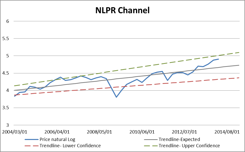
Although the price seems to approach the higher end of the channel, we believe that, based on historical tendencies, the probability is greater for the price to continue trending toward the upper confidence level and linger before finally coming down. Out of the 41 total quarters measured, price oscillated above the gray "expected" trendline for 22 quarters, or 54% of the time. The last period during which price approached the upper end of the channel, in 2006, price remained within an average range of 0.4% variation from the upper confidence level, for 6 quarters. Furthermore, the average duration of a bull cycle (when the price is above the "trendline-expected") is 5.5 quarters, while the average duration of a "confirmed" bull cycle (when the logged price is within 2% or less below the "trendline-upper confidence"), such as the one in 2005-2007, is 8 quarters. The current bull cycle began in the first quarter of 2013, as IYT is approximately 5 quarters into the cycle (3 quarters below the average/previous confirmed bull cycle), while the logged price as of close of trading in June 2, 2014 is approximately 1% below upper confidence level of the channel. Hence, in a "confirmed bull-cycle" environment such as the current one, we expect that price will continue to move to the upper end of the channel over the next 3 quarters, implying a value of 5.076 or $160 per share toward the end of 2014.
Technical Model | |
Trendline-Upper Confidence FY 2014 | 5.076174733 |
Implied Price | $ 160.16 |
Conclusion
The Battle of Price vs. Value
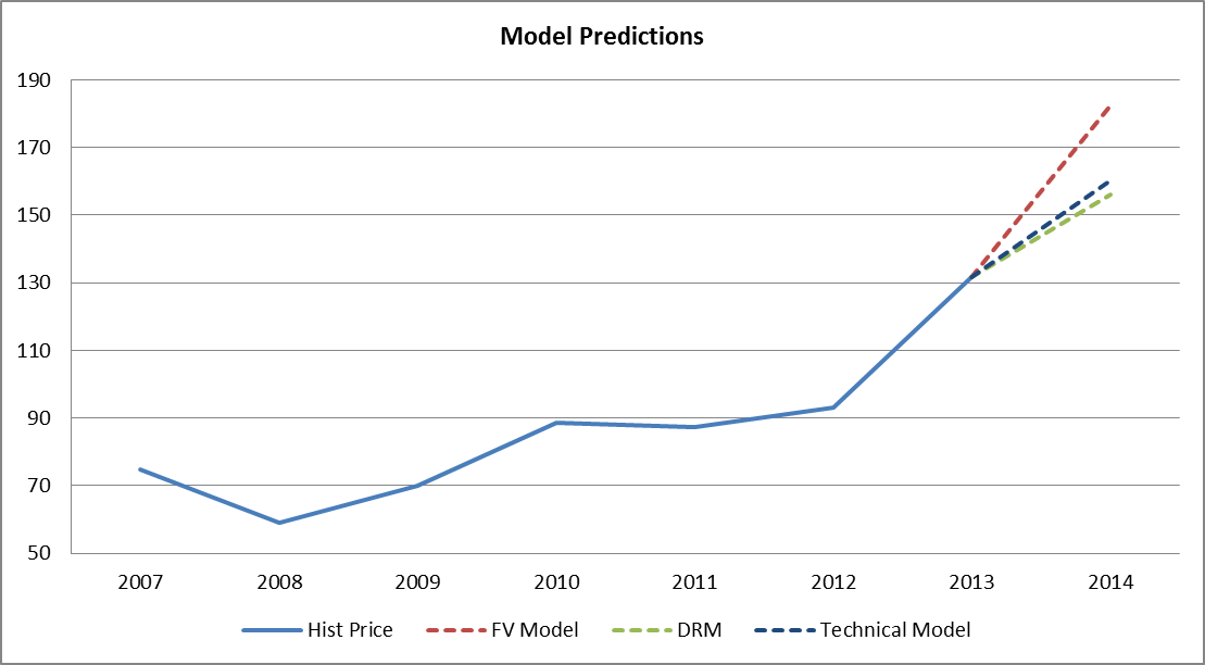
Although its price has risen substantially, and has been making new highs throughout 2013 and the first half of 2014, the iShares Dow Jones Transportation Average ETF still has some way to travel before the end of the route. Fundamentally, a steady disposable income and inflation, along with a weaker dollar will be able to boost durable goods consumption and manufacturing, thus paving the way for gradual growth in the freight industry. Supplemented by evident cyclicality within the industry, the assessed macro drivers are expected to steadily enhance freight quantity, while price stability will allow revenue growth to outpace the growth of costs, resulting in a 5-year average annual growth rate in earnings of approximately 20%. Our fundamental model projects that at this rate, the fair value for the ETF's NAV will be approximately $1.343 Billion at 2014 year-end, translating into a price target of $182 per share. Comparing the growth of total freight expenditures to the change in IYT's price directly, we arrive at a target of $156 per share, but it is important to note that with this method, we overlook the impact of operating costs fluctuation (precisely the reason why we give this model the lowest weighting). On the technical side, as price is currently in a "confirmed bull cycle," we expect that it will continue moving along the upper confidence level of our NLPR Channel with a target of $160 per share for the end of 2014. We weight the fundamental valuation model, the direct approach model, and the technical model 45%, 15%, and 40% respectively, as the premise is that fundamentals account for a majority of the medium and longer term price performance, while momentum takes the stand in the short and shorter-medium term. Hence, based on our fundamental and technical outlook, the weighted average price target for IYT by the end of 2014 is $170 per share.
Model Targets and Weights | ||
Model | Weight | Price Target |
FV Model | 45% | $ 182.42 |
DRM | 15% | $ 156.04 |
Technical Model | 40% | $ 160.16 |
Weighted Average | 100% | $ 169.60 |
Downside Risks
We see possible macro risks to our price target, concerning ECB plans for further easing, which implies a relative strength in the U.S. Dollar relative to the Euro. In addition, a possible pick-up in U.S. inflation above 2.3% (annualized) would also prove a downside risk to our valuation.
Furthermore, we see sub-industry specific risks, primarily associated with federal regulation affecting the freight industry, both directly and indirectly. In particular, the movement toward "green" or "environmentally friendly" products implies a continuation in the decline in volumes of coal and related products, affecting rail freight companies directly.
Possibility for the introduction of drones in the delivery services sub-industry would imply competition pressures to FedEx, UPS, and Expeditors.
Upside Risks
Upside risks include the investment in fuel-efficient trucks and locomotives implying higher fuel savings for rail and trucking companies. Fuel efficiency will have a higher impact on the trucking industry, as rail companies such as Union Pacific implement a charge mechanism which forces clients to cover a certain portion, pegged to a benchmark, of fuel costs.
New technology in the automotive industry, has strong implication for insurance costs in the trucking industry, as implementation of automation such as Peloton Technology's "platooning system" have the potential to substantially reduce insurance costs.
Disclosure: I have no positions in any stocks mentioned, and no plans to initiate any positions within the next 72 hours.