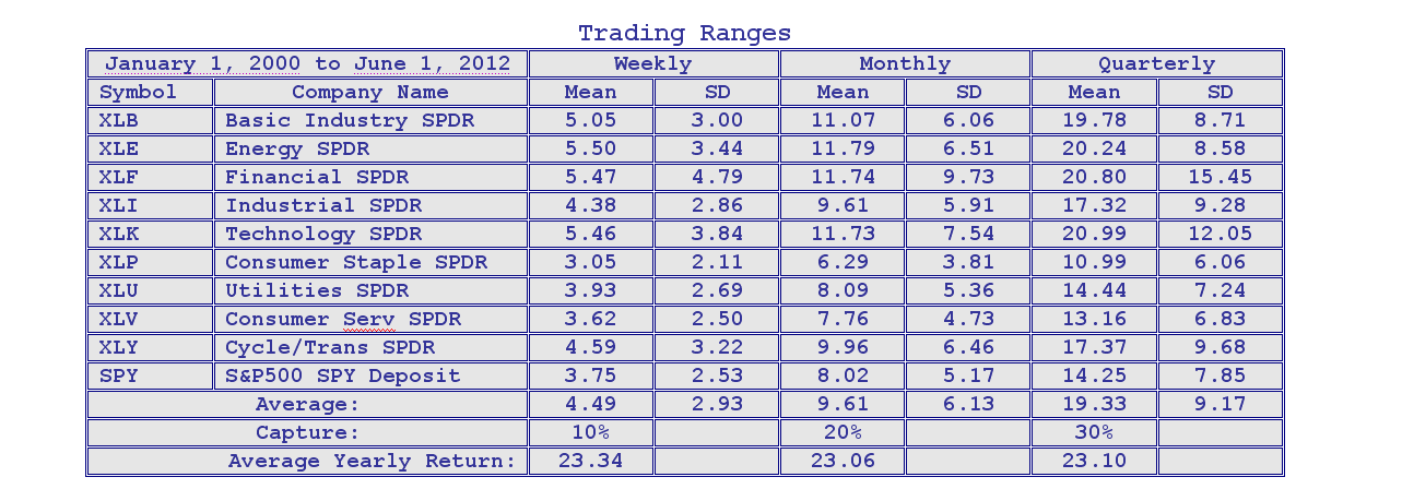
Control Risk and Captured Return: The table below lists the average weekly, monthly and quarterly trading ranges for the 9 Economic Sector ETF's and the SPY from January 1, 2000 through June 1 2012.
Let's say you had a dependable investment strategy that could capture 10% of the Weekly Trading Range. Even capturing a small percent of the available range adds up to an attractive average return of +23.34% per year. Suppose you wanted to limit the number of adjustments to a maximum of 12 per year. So, you reset the process to capture 20% of the monthly volatility instead of 10% of the weekly volatility. Your average return would be approximately the same + 23.06%.
Finally, with a little more capture and half as many adjustments, you have optimized the process to capture the same dollar amount of price fluctuation per year.
The Tactical objectives of the program:
- Limit Risk to a static maximum of 4% per SPDR Position
- Limit the number of adjustments to 4 to 5 per year
- Capture 30% of the Quarterly price range.
- Average a return of 23.10% per year.
- Modest turnover.
The Strategic Goals:
- Full protection for each asset
- Participation in the price movements of each issue
- Capture both Positive and Negative volatility - equally
- Accumulate profits within a secured cash pool for timely distributions.
- Modest Turnover of < 30%
The success of this investment strategy is dependent upon two sets of skills. The first is the ability to recognize the future price momentum of the underlying ETF. The second is to have the know-how to put into action the "best-fit" option strategy that will capture the most amounts of gains with the least amount of risk.
It's well known that the future price movement of an ETF is completely dependent upon the future price movements of the majority of its weighted components. It stands to reason that if one could some how accurately predict the most probable price direction for all 500 of the weighted components of the S&P500 Index, then the next logical step would be to apply these forecasts into a model that could be used toward predicting the price momentum of the SPY.
Let's start by taking a step back and looking at the "big picture". Envision yourself hovering above a 14 year weekly bar chart of the S&P500 Index. Moving from left to right you will see 5 elongated trading channels. The 1st is an ascending channel the starts prior to 1998 and ends at the beginning of 2000. This is followed by a descending channel that starts in 2000 and ends in 2003. The next channel ascends for about 4 years and ends at the end of 2007. After that, the S&P500 Index collapses into a deep decline ending its drop in March of 2009. The 5th channel starts its ascent at the March 2009 low and continues within its ascending pattern to the present.
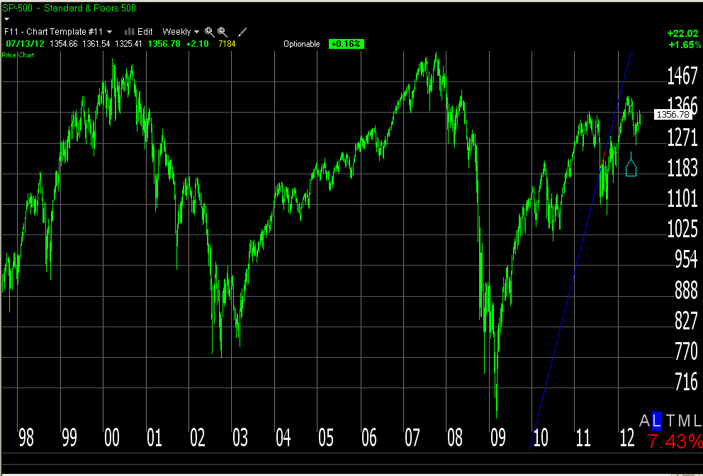
Copyright Worden Brothers TC-2007
Now, move closer to the bar chart and zoom in on one of the long term trading channels. You will find embedded within this channel a series of alternating patterns of ascending/descending trading channels. Next, take out a magnify glass and you will find that the same series of patterns are iterated through out the data all the way down to the tick by tick trades.
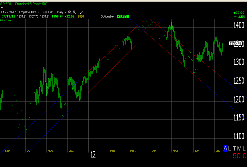
Copyright Worden Brothers TC-2007
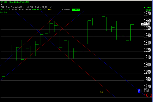
Copyright Worden Brothers TC-2007
What you just uncovered is that long term momentum is derived from the price structure of shorter term trading channels that are continuously found within shorter and shorter time frames all the way down to the "tic by tic" trades found within an intraday trading chart.
We theorized that if we could somehow quantify the short term data stream we would have a foundation to build it out into a longer term momentum indicator. So we wrote a program that created a continuous data stream from daily range data which was then broken into a series oscillating price ranges. Each range has its own magnitude, so that each successive range is either greater than or equal to or less than the previous range. A set of four consecutive bars creates a universe of 16 possible combinations: 8 Positive 8 Negative. Each configuration can only evolve into one of two possible next configurations. We applied the theory of numbers and ran a test over 10 years of daily data for more than 7500 issues. This created a sample in excess of 7.5 Million 4 bar combinations.
The data was then sorted into the 16 possible 4 bar configurations and the program took this data and used it to define the likelihood of the "Next" configuration based upon the magnitudes of the previous four price bars. The outcome was profound. It verified what we saw while hovering over the 14 year daily price chart of the S&P500 Index. This was that each issue spends 71% of the time trading within either an ascending or descending trading channel.
So we built a model predicated on fact that an ETF will always move in the same direction as the majority of it weighted components and that we had a methodology to measure the most probable price path that each of these components was likely to travel.
We built a model that combines the calculations within three time frames:
1-5 Days Momentum
5-25 Days Momentum
2 to 6 weeks Momentum
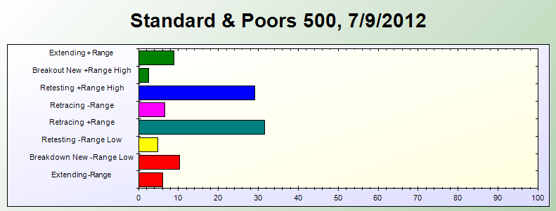
The 1-5days data is color coded:
Bullish
- Green Bars - Extending
- Blues Bar - Retesting - Cautious
- Teal Bar - Retracing
Bearish
- Red Bars - Extending
- Yellow Bar - Retesting - Might reverse
- Pink Bar - Retracing
The 5 to 25 days indicator measures all the weighted components that are trading within 5-25 day trading channels. The green plot is the weighted measurement all the issues that are within ascending channel minus the weight of all the components trading within descending channels.
The 2 to 6 Week Momentum Indicator measures all the weighted components that are trading within 2 to 6 weeks trading channels. The Red Plot is the weighted measurement all the issues that are within ascending channel minus the weight of all the components trading within descending channels.
Now that we have defined a method which we can confidently use to quantify the price momentum of an ETF, the next step toward developing a successful investment program is to develop a simple option's strategy that would effectively capture a certain percentage of an ETF's price movements, while controlling risk. We will use a combination of listed put contracts to capture the upside price changes, and listed "Short" call contracts to capture the downside volatility. We'll use the SPY as our underlying asset.
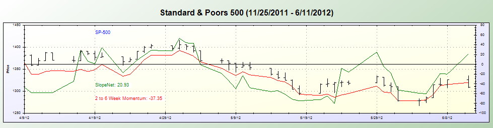
Let's go back a few weeks and take you through a real example. On 6/11/2011, the majority of the weighted components for the S&P500 Index were trading within ascending trading channels as shown by the green line in the chart below( SlopeNet= +20.83). This implies that the momentum for the S&P500 Index is shifting toward a positive direction.
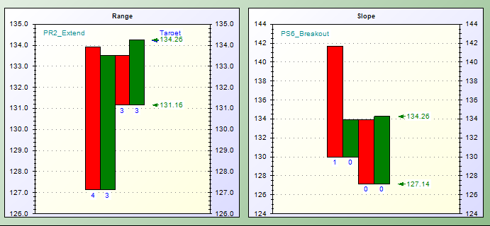
On 6/15/2012, the Positive Momentum was confirmed by the next two significant events. One, the majority of the weighted components within the S&P500 Index were, for the first time since the end of April, trading within "2 to 6 Week Trading Channels" (Red line). Second, the Price Structure of the SPY began trending within its own Positive Slope Configuration (synonymous with a Positive Trading Channel.) This is as bullish as it gets, and will remain so until one and then all of the Indicators change their direction and move into negative territory.
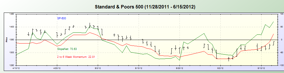
The SPY Price Structure: Range is a "1-5 days" Trading Channel while Slopes are "5 to 25 days" Trading Channels.
Our primary investment objective is to control risk, and we decided at the onset to set the risk bar to a maximum of 4%. On June 15, 2012, the closing price for the SPY was 134.11. The maximum amount of "Married Put Risk" we are allowed to take would have been (0.04)*(134.11) = $5.36.
The following day the SPY opened at 133.59 and the Sept 134.00 Put was selling at $5.68. So if we purchased both at the same time our cost would have been 139.27. The maximum risk would be (139.27 - 134.00) = 5.27 or -3.78%. We are OK.
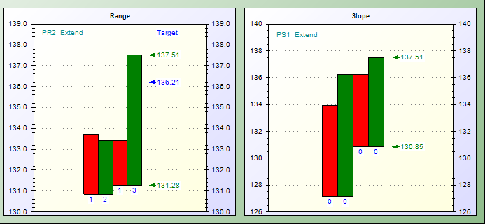
On 7/3/2012 the SPY reached a daily high of 137.51. The "Married Put" combination was worth 140.79 as the September 134.00 Put had dropped in price to $3.28. The August 138.00 Put had also dropped in price to $3.07. If we were to "Roll" the September Put contract "up" 4 strike prices and "in" one expiration date, the cost basis of the position would remain the same, but the maximum risk would drop significantly from -3.78% to (139.27-138.00 Strike) = -1.27 Pts or -1%. In essence, this maneuver would have captured a large portion of the price change as it would have reduced the risk structure from -3.78% to -1.00%.
We are going to use listed call options to capture the downside price changes of the underlying, by selling "short" call contract against a "Married" put position. In the earlier days of my career this formation was referred to as a "Wrap," as in wraps around the underlying, but has since been renamed a "Collar". Let us go through an example of how this strategy works:
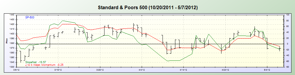
On 5/7/2012 the majority of the S&P500 Index's weighted components were trading within descending trading channels as both the SlopeNet (-18.57) and the "2 to 6 Week Momentum"(-8.25) had moved into Negative territory. Simultaneously, the SPY was caught within its own negative trading configuration as the slope breached its last low. This is as bearish as it gets and will remain so until one and then all three indicators reverse their direction and then move into positive territory

The closing price for the SPY on 5/7/2012 was 137.10. Keeping within the same risk restriction of 4% maximum, we are therefore allowed to take (137.10)*(0.04)= 5.48 points of risk. The next day the SPY opened at 136.31. The July 137.00 Put was selling at $4.29, and the July 130 Call was selling at $9.10.
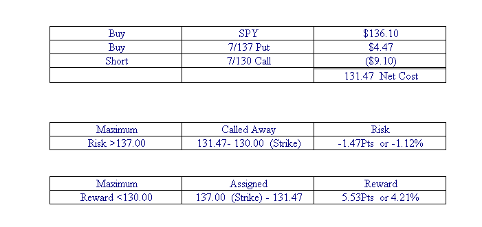
It is important to keep in mind that the objective of this options strategy is to capture volatility and convert it into a capital gains cash flow. It is not likely that any of these positions will go into expiration. However, the program always spells out the worst-case scenario which always means that the position remains unchanged into expiration.
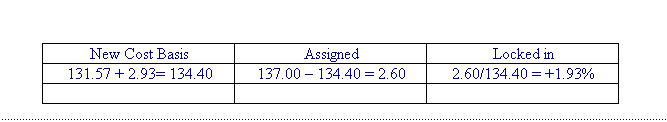
On 6/5/2012, the SPY reached a daily low of 127.14 which was an 8.96 point drop from where we had bought the original position. The July 130 call option was selling at $2.93. If we went ahead and bought back the Call Option we would have captured $6.17, or 69% of the price drop. By buying back (covering) the call option, we essentially lowered the cost basis of our original "Married Put" position to 134.40 and locked in a guaranteed return of +1.93% if we chose to deliver upon our put contract
This is a simple investment strategy that works pretty well. It can be applied to individual stocks as well as to a customized equity portfolio. This is a strategy that allows a portfolio manger to mitigate risk and remain fully invested.
I will post a daily Instablog with a current prognosis.
Disclosure: I am long SPY.
Additional disclosure: I actively advise on similar positions